Grouped GEMM for Imbalanced Experts on Blackwell: A WIP Worklog
This post is a worklog on implementing and optimizing a ragged- grouped GEMM on an NVIDIA B300. It is a work in progress, and I hope to add continuations as I explore the Blackwell architecture more deeply.
Why grouped GEMM?
GEMMs found in Mixture-of-experts are heavily dependent on the number of tokens each expert caters to. This turns an otherwise regular matrix multiplication into an irregular scheduling problem as the distribution of tokens can be highly skewed. For a given expert-FFN projection, expert computes:
Here, and remain fixed, while - the number of tokens routed to expert - varies at runtime. The expert-FFN projections can therefore be executed as ragged- grouped GEMMs. Their performance depends on:
- routing skew and the resulting distribution of work across experts;
- tail waste and effective -tile utilization;
- how tiles are scheduled across the GPU;
- register and shared-memory footprints, which can constrain CTA residency and latency hiding;
- data-movement and instruction overhead;
- achieved tensor-core utilization and throughput.
Having written a few dense GEMM kernels, I wanted to understand which hardware optimizations would transfer to this workload, which ones would regress, and where writing inline PTX would become useful - or necessary - to directly exercise lower-level Blackwell instructions such as tcgen05.
What this worklog covers
The implementation progresses through three kernels:
k0: FP32 CUDA Baseline
A straightforward implementation using scalar FP32 FMA instructions and a flat work schedule.k1: Synchronous Tensor-Core kernel
A warp-tiled implementation built aroundmma.sync, followed by experiments with tile sizes, scheduling, occupancy, and fragment double-buffering.k2: Asynchronous Blackwell kernel
A design using TMA,mbarrier-based synchronization, warp specialization, and a multistage shared-memory pipeline.
Across these three kernels, useful throughput improved by 20.6× under uniform routing - from 21.4 to 440.1 TFLOP/s - and by 17.8× at skew - from 20.1 to 357.0 TFLOP/s. This is still roughly 20% of the B300’s nominal dense BF16 Tensor Core peak of 2.25 PFLOP/s per GPU. Evidently, there's a lot more to explore. I heavily used profiler measurements to understand why seemingly useful optimizations sometimes made the complete kernel slower. I used profiler measurements - including tensor-core utilization, instruction count, register pressure, occupancy, and scheduler stalls - to understand how tile shape, pipeline structure, and routing-induced tail waste affected throughput.
A recurring theme was improving a local metric - such as load latency or pipeline depth - does not necessarily improve overall kernel throughput.
I repeatedly found myself going to Aleksa Gordić’s Inside NVIDIA GPUs: Anatomy of High-Performance Matmul Kernels. It made several aspects of the Blackwell architecture significantly less convoluted, and I strongly recommend it to anyone beginning to write high-performance kernels.
For transparency, the implementation, experiments, profiling, and measurements presented here are based on code I wrote and ran. I used GPT-5.6 Sol to generate most of the figures from that code, and Grok 4.5 for brainstorming portions of the write-up and explanatory code comments.
What I am measuring. I start after routing, with the input rows already grouped by expert. The kernel computes independent GEMMs , with runtime-decided and imbalanced , in one launch. I leave out routing, scatter/gather, the activation and the second projection. In this harness each token selects one expert, so the token count is also the number of routed rows, .
Contents
- Some Results First
- The Grouped Problem and the Flat Tile List
- FP32 FMA Kernel
- Moving the Math onto Tensor Cores
- TMA and Warp Specialization
- Routing Skew and Tile Utilization
- Next: tcgen05 and Adaptive BM
- Appendix A: Master Results
- Appendix B: Per-Variant Hardware Profile
- References
1. Some Results First
Kernel config parameters for this implementation: bf16 inputs and fp32 accumulation; unless stated otherwise, , , , and there are 16,384 tokens.
| Kernel | 16k · s=0 | 16k · s=1.2 | 2k · s=0 | Best |
|---|---|---|---|---|
| k0 smem FMA | 21.4 | 20.1 | ~9 | 4.9% |
| k1 · BM=128 | 224.2 | 182.3 | 63.9 | 51% |
| k1 · BM=64 | 245.1 | 227.7 | 128.0 | 56% |
| k1 · BM=32 | 178.0 | 162.2 | 154.1 | 40% |
| k1 · BM=64 · FRAG_DB | 218.0 | 193.8 | 68.7 | 50% |
| k2 · S=3 | 393.4 | – | – | 89% |
| k2 · S=2 | 440.1 | 357.0 | 111.1 | 100% |
The corresponding changes were:
- k0 smem FMA: three-level tiling on fp32 CUDA cores.
- k1 · BM=128: tensor cores via
cp.async,ldmatrix, andmma.sync. - k1 · BM=64: a register boundary gives 2× occupancy with less padding.
- k1 · BM=32: the highest issue rate, but more staging work.
- k1 · BM=64 · FRAG_DB: explicit fragment double-buffering experiment.
- k2 · S=3: TMA, an
mbarrierring, and a producer warp. - k2 · S=2: one fewer stage, 29 fewer registers, and two blocks per SM.
All numbers are useful TFLOP/s: , or 90.2 GFLOP per launch at 16k routed rows. The hardware executes additional FMA or MMA work at partial M tiles; section 2.1 separates that scheduled work from useful work. The 2k results also show why the fastest tile at 16k is not necessarily the right tile for a smaller batch.
Useful B300 details to remember
Per SM: 4 schedulers · 64K 32-bit registers, allocated in 256-register warp units · 228 KiB shared memory · 64 warps max · ~1.94 GHz in these runs.
mma.syncis the warp-scoped tensor-core path used by k1 and k2;tcgen05is Blackwell's fifth-generation tensor-core interface.
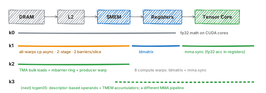
Fig. 1: Kernel progression from 21 to 440 TFLOP/s. k1 moves the arithmetic onto tensor cores. k2 replaces the consumer warps' global-to-shared copy loops with TMA and coordinates the shared-memory stages with mbarriers. k3 will replace the warp-scoped ldmatrix + mma.sync path with tcgen05.
2. The Grouped Problem and the flat tile list
With Simon Boehm's How to Optimize a CUDA Matmul Kernel for cuBLAS-like Performance: a Worklog and Pranjal Shankhdhar's Outperforming cuBLAS on H100: a Worklog covering all the machinery needed to write dense GEMM kernels that outperform cuBLAS, grouped GEMM felt like a good next problem: close enough to reuse the same machinery, but with ragged experts adding enough quirks to make it interesting to optimize. After routing, one multiplication becomes independent GEMMs . Each is known only at runtime, and every expert rounds up independently to the M tile size.
Instead of launching one kernel per expert, I flatten all output tiles into one expert-major descriptor list and launch it once. Each block reads one descriptor and computes one tile. This removes the per-expert host launches and gives the GPU scheduler a single grid containing tiles from all experts.
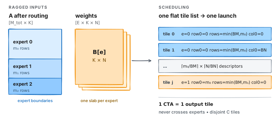
Fig. 2: The grouped problem and its flat tile list. Each descriptor maps one block to one expert and one output tile. The block owns that tile and completes its full K reduction, so no cross-block reduction is needed. I stop tiles at expert boundaries because rows assigned to different experts use different weights; crossing a boundary would make one block compute pieces of two GEMMs. As the routed-row count changes, only the descriptor list and launch grid change.
Source — k1/common.cuh · k1/harness.cu: tile descriptor and enumeration
struct Tile {
  int expert;  // B[expert]
  int row0;    // row offset in A and C
  int rows;    // valid rows in this tile
  int col0;    // column offset in C
};

for (int e = 0; e < a.E; ++e)
  for (int mt = 0; mt < cdiv(m_e[e], BM); ++mt)
    for (int nt = 0; nt < cdiv(a.N, BN); ++nt)
      tiles.push_back({e, (int)off[e] + mt * BM,
                       std::min(BM, m_e[e] - mt * BM),
                       nt * BN});
2.1 Skew and tile efficiency
To emulate imbalanced expert loads, I use a power-law skew parameter to control how many routed rows
each expert receives: expert receives rows in proportion to
. At , the rows are distributed evenly. At , the largest
expert gets 4,793 rows and the smallest gets 32. Every block still executes the full compute loop. The
t.rows guard prevents rows beyond the current expert from being stored. In k2, TMA can still fetch rows
beyond the logical expert boundary. In all three kernels, a partial tile executes the same FMA or MMA loop as a
full tile.
I use for the fraction of scheduled rows that contain valid routed rows. It captures the padding introduced by a particular expert distribution and BM:
To estimate throughput under skew from a balanced run at the same workload size, kernel, and , I use:
For example, k2/S2 gives TFLOP/s at skew 1.2. The measured result is 357.0 TFLOP/s. accounts for the additional full-tile arithmetic created by partial tiles. It does not model per-CTA staging, synchronization, and scheduling overhead, finite-grid effects, occupancy changes, or cache behavior.
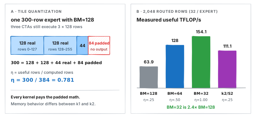
Fig. 3: Tile quantization in the grouped GEMM. An expert's last partial tile consumes a full tile's compute. Router skew and small batches therefore reduce row utilization. At 16k, BM=32 is slower than BM=64 and BM=128 because it creates more tiles and repeats B staging and synchronization more often. At 2,048 evenly distributed routed rows, each expert receives exactly 32 rows. BM=32 has no row padding, while BM=64 and BM=128 pad 50% and 75% of their row compute. BM=32 therefore reaches 154.1 TFLOP/s, 2.4× BM=128's 63.9 TFLOP/s.
Here is how the -only estimates compared with the measurements:
| Config | Estimate | Measured | |
|---|---|---|---|
| k1/128 · 16k · s=1.2 | 0.780 | 182.3 | |
| k1/128 · 2k · s=1.2 | 0.225 | 58.0 | |
| k1/64 · 16k · s=1.2 | 0.898 | 227.7 | |
| k2/S2 · 2k · s=0 | 0.250 | 111.1 | |
| k2/S2 · 16k · s=1.2 | 0.780 | 357.0 |
must be recomputed for every BM. At skew 1.2, BM=64 wastes 10.2% of its scheduled rows; BM=128 wastes 22.0%. BM therefore controls the cost of skew as well as the cost of small batches.
In the k1 skew sweep, DRAM traffic stayed around the ~474 MB compulsory total. Issue-active still rose from 44.65% to 45.93% while useful throughput fell: more of the issued math was multiplying padded rows.
How I measure. Compile with
-Xptxas -vto check register usage and spills. If there are spills - I would say it's a strict No. As for the profiler, I usedncuto get the tensor-core utilization, instruction count, pipeline depth, occupancy, and scheduler stalls.
Remember to skip sufficient launches for warmup.
ncu --launch-skip 11 --launch-count 1 <program>
This skips one correctness launch and ten warmup launches, then profiles one timed launch.
3. I started with a naive fp32 FMA kernel: 21 TFLOP/s
In the first kernel, I implemented a simple tiled GEMM to test the flat tile list, expert offsets, and partial tiles at expert boundaries before adding tensor cores and asynchronous copies. It uses a 64×64 shared-memory tile with K-slices of 16. Each of the 256 threads owns a 4×4 register micro-tile and performs rank-1 updates. The global inputs are bf16; the shared-memory tiles and arithmetic are fp32.
Source — k0/k0_tiled.cuh: shared-memory tile and inner loop
__shared__ float As[BM][BK + 1];
...
#pragma unroll
for (int kk = 0; kk < BK; ++kk) {
  float a[TM], b[TN];
  for (int i = 0; i < TM; ++i) a[i] = As[ty * TM + i][kk];
  for (int j = 0; j < TN; ++j) b[j] = Bs[kk][tx * TN + j];
  for (int i = 0; i < TM; ++i)
    for (int j = 0; j < TN; ++j) acc[i][j] += a[i] * b[j];
}
At 16,384 routed rows, the kernel reached 21.4 TFLOP/s with uniform routing and 20.1 TFLOP/s at skew 1.2. Throughput dropped to about 9 TFLOP/s at 2,048 routed rows and remained at 21.0 TFLOP/s when K increased to 8,192. The kernel used 56 registers per thread and 9 KiB of shared memory per block, permitting four 256-thread blocks per SM.
I verified the tile counts with the descriptor enumeration. k0 uses 64×64 tiles, including 42 tiles along N, and
logs tiles=10752/11970 for balanced/skewed 16k runs. All the runs match
as well: 10,752 for k1/32 at balanced
16k and 2,688/3,444 for k2 at balanced/skewed 16k. At balanced 2k, k1 and k2 use 1,344 descriptors because
BN=128; k0 uses 2,688 because BN=64.
A naive implementation only achieves around 21 TFLOP/s, about 25% of the 79.5 TFLOP/s peak of fp32 CUDA cores. However, since the BF16 tensor-core ceiling is more than an order of magnitude higher, it made sense to move on to a variant that could leverage the 2.25 PFLOP/s it provides.
4. Moving the Math onto Tensor Cores: 20.1 → 227.7 TFLOP/s at
For k1 I used an Ampere-style tensor-core design: a 128×128 block tile, eight warps arranged as a 2×4
grid of 64×32 warp tiles, and a two-stage shared-memory buffer filled with per-thread
cp.async. ldmatrix moves each fragment from shared memory into the registers expected by
mma.sync.m16n8k16, with bf16 operands and fp32 accumulators.
4.1 Fragment layout: ldmatrix and mma.sync
The BF16 m16n8k16 form of mma.sync was introduced with Ampere (sm_80). It is a warp-level operation: all 32 lanes collectively compute a matrix multiply-accumulate using register-resident fragments distributed across the warp. For this instruction, each lane provides eight BF16 elements of , four BF16 elements of , and four FP32 accumulator elements, following a fixed lane-to-element mapping defined by the PTX ISA. ldmatrix collectively loads the shared-memory tiles into the register layout expected by the MMA instruction.
WMMA keeps fragment layouts opaque and does not support the m16n8k16 shape, so I use
mma.sync PTX directly. This exposes the lane-to-register mapping, allowing the epilogue to store each
accumulator directly to its corresponding position in C, without staging the output tile through shared memory.
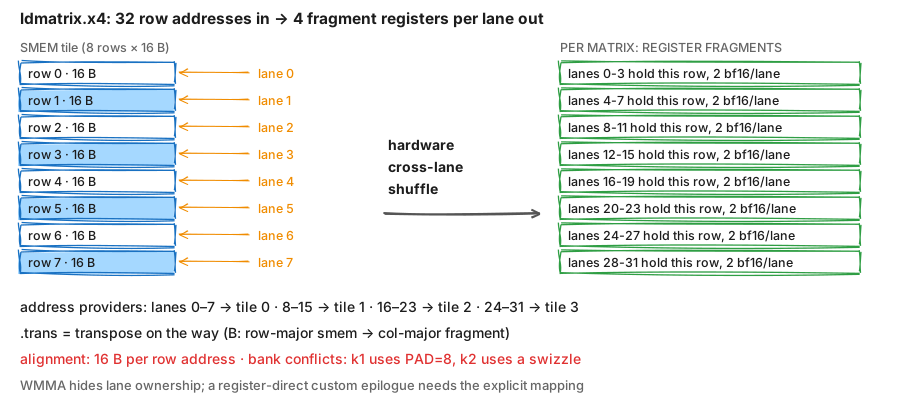
Fig. 4: The ldmatrix contract, step by step. Each 8×8 b16 tile is 8 rows × 16 bytes. Every lane supplies the smem address of one 16-byte row (lanes 0–7 give tile 0's rows, 8–15 tile 1, and so on); the hardware does the cross-lane shuffle and each lane ends up holding its mma-layout slice. .x4 means four tiles, 512 B per warp per instruction. The .trans variant transposes on the way (needed for B: mma wants col-major, smem holds row-major).
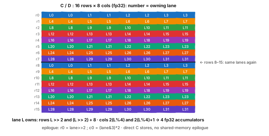
Fig. 5: The C/D accumulator layout across all 32 lanes. The tile is 16×8 fp32; colors mark lane groups of four and each cell contains its owning lane. Every lane holds four values: a pair of columns at row L >> 2 and the same pair at (L >> 2) + 8. The epilogue uses this mapping to store the accumulator registers directly to C.
Source — k1/k1_cpasync_mma.cuh: fragment addresses and the register-direct epilogue
// A fragments (16 rows x 16 k): lanes 0-15 pick the row, lanes 16-31 the second k-half
&s.A[buf][wm + mi*16 + (lane & 15)]      // (lane & 15): one 16-byte row-chunk per lane
          [ks*16 + ((lane >> 4) << 3)]   // (lane >> 4): 0 or 8 -- which 8-col half
// B: same contract + .trans (mma is row.col; smem B is row-major)
&s.B[buf][ks*16 + (lane & 15)][wn + nb*16 + ((lane >> 4) << 3)]

// Epilogue coordinates from Fig. 5
const int r0 = wm + mi*16 + (lane >> 2);
const int c0 = wn + ni*8  + (lane & 3) * 2;
...
if (r >= t.rows) continue;
For ldmatrix.m8n8.b16, one lane supplies each naturally aligned 16 B row address;
the returned row is distributed across a group of four lanes. Bank conflicts are a separate performance
constraint: k1 changes the
row stride with PAD=8, while k2 uses the 128 B swizzle in Section 5.3. In
mma.sync.m16n8k16, each lane contributes 16 B of A and 8 B of B; narrower input types increase K
while preserving those operand bytes per MMA.
4.2 Three PTX wrappers
Source — k1/ptx.cuh: cp.async, ldmatrix, and mma.sync wrappers
// cp.async
__device__ __forceinline__ void cp_async_16(void* dst, const void* src, bool pred) {
    const int n = pred ? 16 : 0;
    asm volatile("cp.async.cg.shared.global [%0], [%1], 16, %2;\n"
                 :: "r"(smem_addr(dst)), "l"(src), "r"(n));
}

// ldmatrix
"ldmatrix.sync.aligned.m8n8.x4.shared.b16 {%0, %1, %2, %3}, [%4];"

// mma.sync
"mma.sync.aligned.m16n8k16.row.col.f32.bf16.bf16.f32 "
"{%0, %1, %2, %3}, {%4, %5, %6, %7}, {%8, %9}, {%0, %1, %2, %3};"
4.3 A two-stage cp.async pipeline
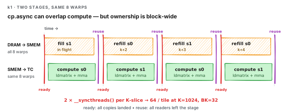
Fig. 6: k1's two-stage pipeline. The double buffer overlaps the next cp.async group with compute on the current stage. Every warp participates in both copying and math, which requires one block-wide __syncthreads() before reading a stage and another before reusing it. At K=1024 and BK=32, that is 64 block barriers per output tile.
Source — k1/k1_cpasync_mma.cuh: the two-stage loop
for (int kt = 0; kt < KT; ++kt) {
  if (kt < KT - 1) cp_async_wait<1>();
  else             cp_async_wait<0>();
  __syncthreads();
  const int buf = kt & 1;
  /* ldmatrix + mma.sync */
  __syncthreads();
  if (kt + 2 < KT) load_stage(s, buf, ..., (kt + 2) * TBK, tid);
}
The first version reached 224.2 TFLOP/s, a 10.5× jump over k0. Its scheduler issue rate and block residency explain the next set of changes.
4.4 Reading the scheduler
Let be the resident warps per scheduler, and let be warp cycles per issued instruction. Then:
With four schedulers per SM:
For the register limit, let be registers per thread and be warps per block. Because registers are allocated to each warp in 256-register units:
Here, is the register-limited number of resident blocks per SM.
Final block residency is the minimum of the register, shared-memory, warp, and architectural block limits. For k1/128, 95 registers allow two whole blocks per SM, and the profiler measured warps per scheduler. With warp cycles per instruction, eq. (2) predicts an issue rate of 0.459. The measurement was 0.46; predicted SM IPC was 1.84 and measured IPC was 1.83.
The kernel was latency-bound and short of eligible warps: the scheduler issued on 46% of cycles. Register allocation happens in 256-register warp units and blocks must land whole, so 95 registers per thread leaves 16K registers unused and yields 16 resident warps. The rounded components in the profiler's stall breakdown also sum to approximately .
4.5 The BM sweep and a register boundary
I templated the kernel over <BM,BN,BK,WM,WN>, shrinking the warp tile with the block tile while
keeping eight warps and 256 threads. With 16k balanced routed rows, every variant has , so this sweep isolates
the hardware rate.
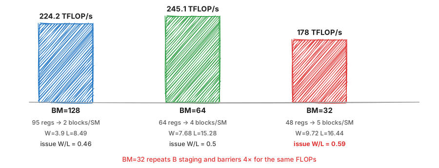
Fig. 7: What changed as I reduced BM. BM=64 lands exactly on the 64-register boundary and allows four blocks per SM. BM=32 produces the highest issue rate and the lowest 16k throughput. Every block still stages the same 32×128 B tile per K-slice, so four times as many blocks bring four times as many B-staging instructions and barriers for the same useful FLOPs. The schedulers are busy, though much of what they issue is setup work.
Source — k1/k1_cpasync_mma.cuh: A and B staging loops
for (int i = tid; i < TBM * TBK / 8; i += THREADS) { ... }   // scales with BM
for (int i = tid; i < TBK * TBN / 8; i += THREADS) { ... }   // fixed for every block
Randomizing the BM=32 descriptor order reduced throughput from 178.0 to 174.4 TFLOP/s, only 2%. Descriptor locality therefore explains only a small part of the gap from BM=64; BM=32 still performs four times the B staging and block barriers for the same useful FLOPs.
4.6 Fragment double-buffering
wait and short_scoreboard contributed about 5.3 cycles per instruction.
short_scoreboard is a dependency on an MIO operation, and the inner loop places
ldmatrix directly before the MMAs that consume its registers. I tested two register-fragment
sets, loading k-step ks+1 before issuing the MMAs for ks. The experiment remains available behind
-DK1_FRAG_DB=1.
uint32_t af[2][TWM/16][4], bf[2][TWN/8][2];                  // ping-pong sets
load_frags(s, buf, 0, af[0], bf[0], ...);                    // prime
#pragma unroll
for (int ks = 0; ks < KS; ++ks) {
  const int cur = ks & 1;
  if (ks + 1 < KS) load_frags(s, buf, ks+1, af[cur^1], bf[cur^1], ...);   // overlap
  /* mma on af[cur]/bf[cur] */
}
The stall numbers improved. L fell from 15.28 to 13.70, the targeted stalls fell from 5.26 to 3.86, and register use dropped from 64 to 56. Throughput still went the other way: 245 → 218 TFLOP/s.
sm__inst_executed.sum increased from 214.35 M to 269.19 M, or 25.6%, because of additional SASS
register moves and address arithmetic. The lower stall cost per issued instruction did not compensate for the
larger instruction stream.
4.7 What still limits k1
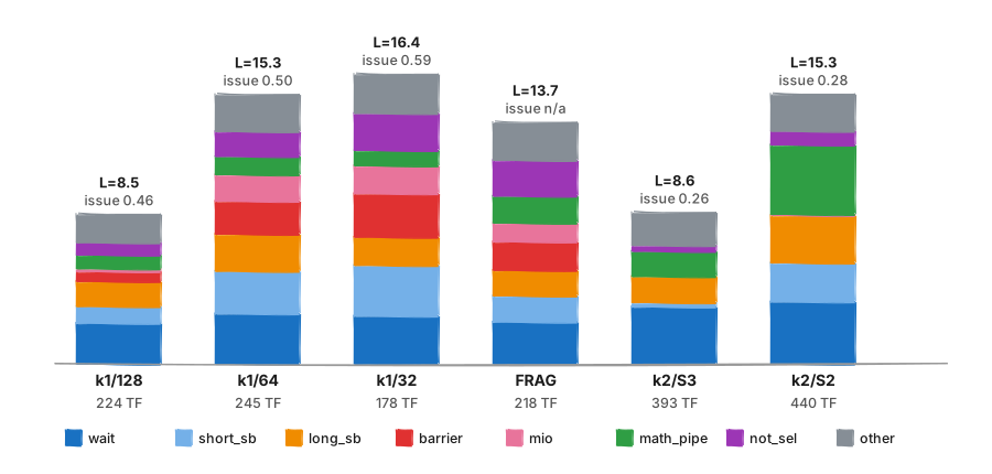
Fig. 8: Warp cycles per issued instruction across the variants. The rounded bars partition warp
latency , with above each bar. not_selected is scheduler delay rather than an execution
dependency. k1/128 has low latency and too few resident warps. BM=64 and BM=32 add warps,
along with more barriers, copies and contention. FRAG_DB lowers L while increasing the instruction count. k2 has
no block-barrier stalls in the main loop; by S2 the largest bar is math_pipe_throttle, meaning the
warp is waiting for a math execution pipe.
At BM=64, barriers, copy work, and issue contention accounted for about five of the fifteen cycles. The costs
were smaller at BM=128 because larger tiles amortize the same setup over more FLOPs, but every k1 variant still
made its compute warps copy data, share LSU issue slots with ldmatrix, and synchronize around the
shared buffers.
5. TMA & Warp Specialization: 227.7 → 357.0 TFLOP/s at
In k2, I retained k1's tensor-core math and added a ninth warp to issue the TMA loads. The eight compute warps
read one shared-memory stage while the ninth warp fills another. I increased BK from 32 to 64 so one row of 64
BF16 values occupies 128 B, matching the TMA swizzle atom. K2_STAGES sets the number of stages in
this circular buffer.
5.1 TMA copy path
TMA is the hardware-assisted asynchronous bulk-copy path behind cp.async.bulk.tensor. On the host,
I encode the tensor shape, strides, tile box, swizzle, and out-of-bounds policy in a CUtensorMap. In the
kernel, one thread supplies the tensor map, coordinates, shared-memory destination, and completion barrier. The
copy is non-blocking; completion is reported by reducing the mbarrier's transaction byte count.
Compared with k1/BM=128:
- The block-wide
cp.asyncstream and its per-thread address arithmetic become three bulk-tensor instructions per BK=64 stage, issued by lane 0. - The consumer warps stop issuing copies alongside
ldmatrix.mio_throttlefalls from 0.16 to 0.01 cycles per instruction, andshort_scoreboardfrom 0.95 to 0.24. The producer warp can fill a future stage while the eight compute warps consume the current stage. TMA replaces the global-to-shared copies; the compute loop still usesldmatrixandmma.sync.waitis 2.31 cycles per instruction in k1/128, 3.24 in k2/S3 and 3.53 in k2/S2. Nsight Compute defineswaitas a fixed-latency execution dependency, so this counter does not identify a specific instruction.
5.2 TMA and mbarrier instructions
Source — k1/ptx.cuh: mbarrier and TMA wrappers
__device__ void mbarrier_init(uint64_t* bar, uint32_t count);
__device__ void fence_mbarrier_init();
__device__ void mbarrier_arrive_expect_tx(uint64_t* bar, uint32_t tx);
__device__ void mbarrier_arrive(uint64_t* bar);
__device__ void mbarrier_wait_parity(uint64_t* bar, uint32_t parity);

"cp.async.bulk.tensor.2d.shared::cluster.global.mbarrier::complete_tx::bytes"
"        [smem], [tmap, {x, y}], [bar];"
Source — k2/k2_tma_ws.cuh: TMA descriptor setup
const cuuint32_t box[3] = {64, BK, 1};                 // one 64-col B panel per issue
cuTensorMapEncodeTiled(&m, CU_TENSOR_MAP_DATA_TYPE_BFLOAT16, 3, (void*)B, dim, stride, box, estr,
                       CU_TENSOR_MAP_INTERLEAVE_NONE, CU_TENSOR_MAP_SWIZZLE_128B,
                       CU_TENSOR_MAP_L2_PROMOTION_L2_128B, CU_TENSOR_MAP_FLOAT_OOB_FILL_NONE);
5.3 The 128 B shared-memory swizzle
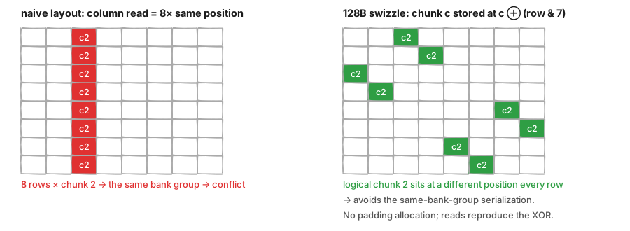
Fig. 9: How distributes an ldmatrix read across shared-memory banks. In the naïve layout, the same 16-byte chunk position in each of eight rows maps to the same four-bank group. The 128-byte XOR swizzle stores logical chunk from row at physical chunk position , distributing the eight accesses across distinct bank groups. k1 changes the row stride using PAD=8; k2 achieves the conflict-free layout without allocating padding.
Source — k2/k2_tma_ws.cuh: swizzled shared-memory address
__device__ __forceinline__ const __nv_bfloat16* swz(const __nv_bfloat16* row_base, int row, int col) {
  return row_base + (((col >> 3) ^ (row & 7)) << 3);
}
ldmatrix_x4(af[mi][0], ..., swz(&sm.A[st][r][0], r, c));
5.4 Connecting the producer and consumers
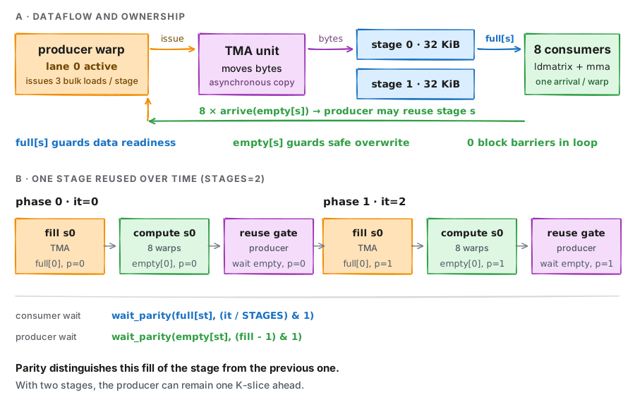
Fig. 10: The mbarrier ring connecting one producer to eight compute warps. The producer issues three TMA loads for stage st. The compute warps wait on full[st], read the stage, and each arrives once on empty[st]. The producer reuses the stage after all eight arrivals. Parity distinguishes successive uses of the same barrier.
Source — k2/k2_tma_ws.cuh: producer and compute-warp synchronization
if (lane == 0) {
  for (int it = 0; it < KT; ++it) {
    const int st = it % STAGES;
    const int f  = it / STAGES;
    if (f > 0) mbarrier_wait_parity(&sm.empty[st], (f - 1) & 1);
    mbarrier_arrive_expect_tx(&sm.full[st], STAGE_BYTES);
    tma_load_2d(&tmapA, &sm.A[st][0][0], /*x=*/it*BK, /*y=*/t.row0, &sm.full[st]);
    tma_load_3d(&tmapB, &sm.B[st][0][0][0], t.col0,      it*BK, t.expert, &sm.full[st]);
    tma_load_3d(&tmapB, &sm.B[st][1][0][0], t.col0 + 64, it*BK, t.expert, &sm.full[st]);
  }
}
// Compute warps
for (int it = 0; it < KT; ++it) {
  const int st = it % STAGES;
  mbarrier_wait_parity(&sm.full[st], (it / STAGES) & 1);
  /* ldmatrix + mma.sync */
  __syncwarp();
  if (lane == 0) mbarrier_arrive(&sm.empty[st]);
}
TMA uses the boundary of the packed A matrix, not the boundary of the current expert. A partial
tile can therefore load rows from the next expert. The t.rows guard prevents those results from being
stored, but the tile still executes the full MMA loop.
The three-stage version reached 393.4 TFLOP/s, 1.75× k1 at the same BM×BN tile size. Barrier stalls read 0.00, and the compute warps no longer carried the copy instruction stream.
5.5 STAGES=2 outperforms STAGES=3
With three stages, the scheduler showed about 65% tensor-pipe utilization but only 2.19 warps per scheduler and 74% of cycles with no eligible warp. Register allocation limited the kernel to one block per SM:
STAGES=3: 123 regs -> 4096/warp x 9 warps = 36,864/block -> floor(65536/36864) = 1 block   (2.19 ~ 9/4, checks out)
STAGES=2:  94 regs -> 3072/warp x 9 warps = 27,648/block -> 2 blocks                        (4.28 measured)
Compiling with two stages reduced register use from 123 to 94 per thread. The aligned shared-memory
allocation fell from 97 KiB to 65 KiB per block. Nsight Compute reported the resulting block limits as
Registers: 2 · Shared Mem: 2 · Warps: 7. Theoretical residency was 18 warps per SM and the
achieved value was 17.11.
With two stages, throughput reached 440.1 TFLOP/s. With two blocks resident, issue moved from 0.26 to
0.28 and L rose to 15.30. The leading stall became math_pipe_throttle at 3.94 cycles, which means the
warp was waiting for a math execution pipe to become available. Speed-of-light metrics reported Compute at 71.9%
and DRAM at 28%.
A third resident block would require 72 registers per thread or fewer; the current kernel uses 94. Further gains require either fewer registers or a different tensor-core path. k3 takes the second route.
6. Routing skew and tile utilization
At 16k routed rows, changing skew from 0 to 1.2 reduces by 10.2% for BM=64 and 22.0% for BM=128. The measured throughput losses are slightly smaller:
| Kernel | TFLOP/s · | Measured | -only |
|---|---|---|---|
| k0 (BM=64) | 21.4 20.1 | −6.1% | −10.2% |
| k1 BM=64 | 245.1 227.7 | −7.1% | −10.2% |
| k1 BM=128 | 224.2 182.3 | −18.7% | −22.0% |
| k2 S=2 (BM=128) | 440.1 357.0 | −18.9% | −22.0% |
predicts only the loss from padded rows. Occupancy, cache behavior, and the number of tail blocks also change between the balanced and skewed grids, so the measured losses do not match it exactly. At 2,048 routed rows, the difference in tile fill is large enough to reorder the variants:
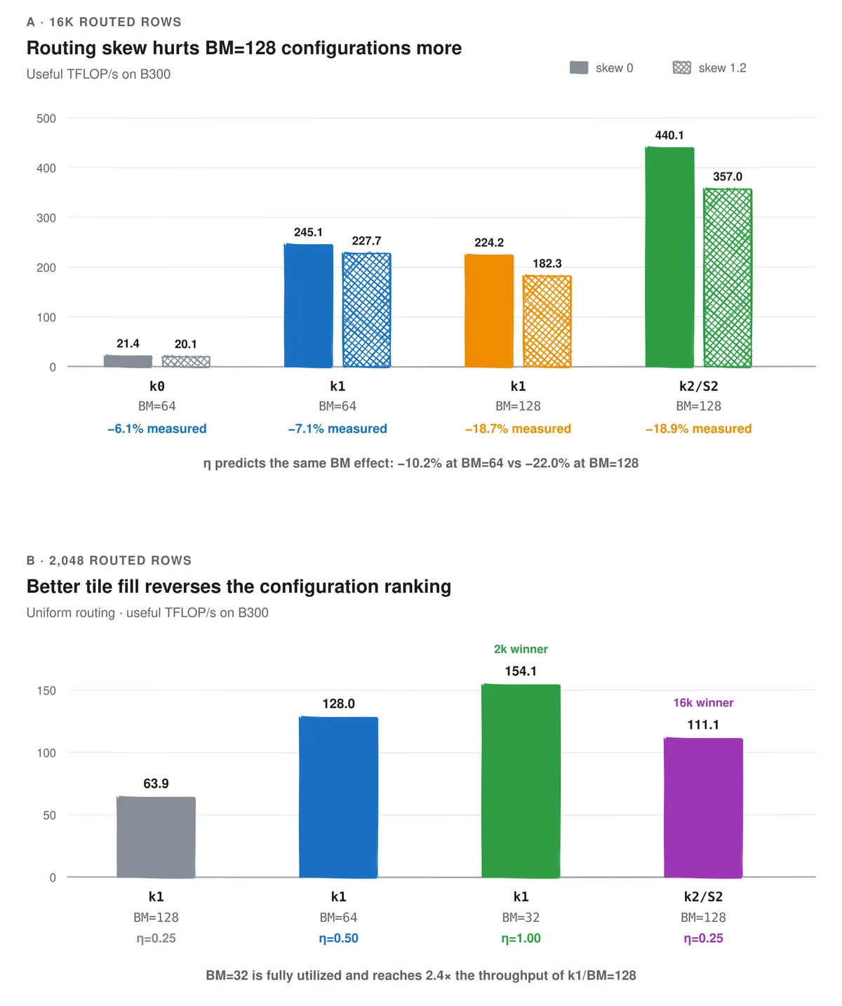
Fig. 11: Tile fill changes the useful-throughput ranking. At 16k, the -only model predicts a 22.0% skew loss for BM=128 and 10.2% for BM=64; all four measurements are three to four points better. At 2,048 routed rows, BM=32 reaches 154.1 TFLOP/s, 2.4× BM=128. k2 reaches 111.1 TFLOP/s against the -scaled estimate of 110.0 from its balanced 16k rate.
A smaller BM reduces padding but creates more tiles and more staging work. BM therefore has to be selected from both the expert sizes and the rate each tile shape achieves. k1 supports BM=32/64/128; k2 still uses BM=128 for every expert.
7. Next: tcgen05 and adaptive BM
The k2/S2 profile reports 3.94 cycles of math_pipe_throttle, with Compute throughput at 71.9% and
L1TEX throughput at 66.9%. Blackwell's asynchronous tcgen05.mma changes this path: A and B can be
sourced from shared memory through descriptors, the accumulator lives in TMEM, and one thread initiates the MMA
for a CTA or CTA pair.
This is a different pipeline from the warp-collective ldmatrix + mma.sync loop, not a
drop-in instruction replacement.
The next version has two separate experiments: replace the register-fragment MMA path with tcgen05,
then choose BM from the expert-size distribution instead of fixing BM=128 for every launch.
Scope of these results. The model, its dependence on BM, the occupancy calculation, and the trade-off between tile size and padding should all apply to GEMMs in MoE. However, the MoE op in general includes more work, including top-k experts, permutation of rows, weighted combination of the expert outputs, and scatter/gather of tokens to experts - and these are missing today. My benchmark also launches the grouped GEMM back to back, which gives it friendlier cache state and one that might differ from a real workload execution which is interleaved with attention and normalization kernels. The numbers in this post describe the grouped GEMM in isolation.
Appendix A: master results
| Kernel | Routed rows | K | Skew | TFLOP/s | ms |
|---|---|---|---|---|---|
| k0 | 16384 | 1024 | 0 | 21.4 | 4.213 |
| k0 | 16384 | 1024 | 1.2 | 20.1 | 4.498 |
| k0 | 16384 | 8192 | 0 | 21.0 | 34.38 |
| k0 | 2048 | 1024 | 0 | ~9 | – |
| k1 BM=128 | 16384 | 1024 | 0 | 224.2 | 0.402 |
| k1 BM=128 | 16384 | 1024 | 1.2 | 182.3 | 0.495 |
| k1 BM=128 | 2048 | 1024 | 0 | 63.9 | 0.176 |
| k1 BM=128 | 2048 | 1024 | 1.2 | 58.0 | 0.194 |
| k1 BM=64 | 16384 | 1024 | 0 | 245.1 | 0.368 |
| k1 BM=64 | 16384 | 1024 | 1.2 | 227.7 | 0.396 |
| k1 BM=64 | 2048 | 1024 | 0 | 128.0 | 0.088 |
| k1 BM=32 | 16384 | 1024 | 0 | 178.0 | 0.507 |
| k1 BM=32 | 16384 | 1024 | 1.2 | 162.2 | – |
| k1 BM=32 SHUFFLED | 16384 | 1024 | 0 | 174.4 | 0.517 |
| k1 BM=32 | 2048 | 1024 | 0 | 154.1 | 0.073 |
| k1 BM=64 FRAG_DB | 16384 | 1024 | 0 | 218.0 | 0.414 |
| k1 BM=64 FRAG_DB | 16384 | 1024 | 1.2 | 193.8 | – |
| k1 BM=64 FRAG_DB | 2048 | 1024 | 0 | 68.7 | – |
| k2 STAGES=3 | 16384 | 1024 | 0 | 393.4 | 0.229 |
| k2 STAGES=2 | 16384 | 1024 | 0 | 440.1 | 0.205 |
| k2 STAGES=2 | 16384 | 1024 | 1.2 | 357.0 | 0.253 |
| k2 STAGES=2 | 2048 | 1024 | 0 | 111.1 | 0.101 |
The k1/32 skew-1.2 and k1/64 FRAG_DB skew-1.2 and 2k measurements were recorded without timings, so their ms cells are blank.
Appendix B: per-variant hardware profile
| k1/128 | k1/64 | k1/32 | k1/64+FRAG | k2/S3 | k2/S2 | |
|---|---|---|---|---|---|---|
| Registers (0 spills everywhere) | 95 | 64 | 48 | 56 | 123 | 94 |
| smem/block | 37 KiB | 27 KiB | 22 KiB | 27 KiB | 97 KiB dyn | 65 KiB dyn |
| Blocks/SM (limiter) | 2 (regs) | 4 (regs) | 5 (regs) | 4 | 1 (regs) | 2 (regs+smem, per ncu) |
| W (warps/scheduler) | 3.90 | 7.68 | 9.72 | – | 2.19 | 4.28 (achieved 17.11/SM) |
| L (cycles/inst, ≍ rounded stall sum) | 8.49 | 15.28 | 16.44 | 13.70 | 8.55 | 15.30 |
| Issue = W/L | 0.46 | 0.50 | 0.59 | – | 0.26 | 0.28 |
| Instructions / launch | – | 214.35 M | – | 269.19 M | – | – |
| SoL SM / L1TEX / DRAM % | 44.7/50.3/14.3 | 49.0/67.1/15.7 | – | – | 64.9/61.0/25.4 | 71.9/66.9/28.0 |
References
Technical references
- NVIDIA, CUDA Programming Guide — CUDA execution and programming model.
- NVIDIA, Parallel Thread Execution ISA —
ldmatrix,mma.sync,cp.async,mbarrier, bulk-tensor copies, andtcgen05. - NVIDIA, Nsight Compute Profiling Guide — stall definitions.
- NVIDIA, Blackwell Tuning Guide — resource limits.
- NVIDIA CUTLASS, Grouped Kernel Schedulers — grouped-GEMM scheduling idioms.
Blogs
- Aleksa Gordić, Inside NVIDIA GPUs: Anatomy of high performance matmul kernels.
- Pranjal Shankhdhar, Outperforming cuBLAS on H100: a Worklog.
- Simon Boehm, How to Optimize a CUDA Matmul Kernel for cuBLAS-like Performance: a Worklog.